Lesson 3: Dynamic and Animated Charts


Introduction

Today, we're going to learn how to build dynamic and animated charts in Excel.

OK, there are two words you already need to clarify, being "Dynamic" and "Animated".

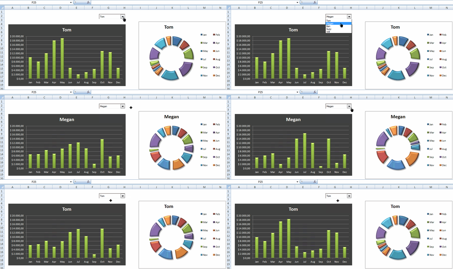
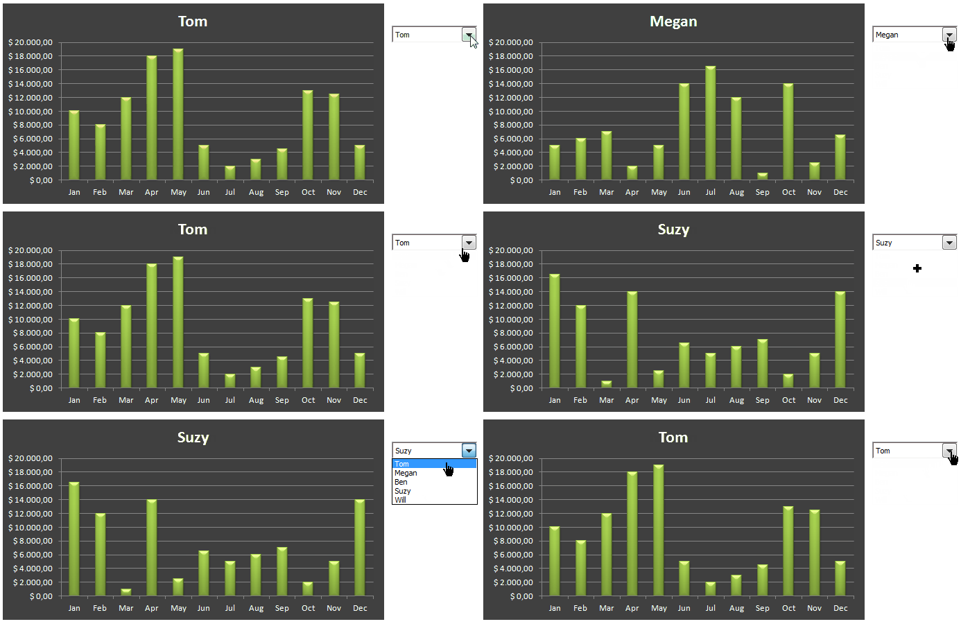
Well, with dynamic we mean that the user can himself choose what data he wants to be plotted on a chart. Animated defines the way the transition between the previous and the current set of information is performed. Instead of having the previous info just being overwritten by the new one, we'll try to add some fluidity. This is what we ultimately want to obtain:


I keep on asking the same question during these lessons, but again, why would I need that?

Just because data is NOT everything. The way data is presented and organized will as well provide a lot of added value. Creating a nice user experience is an important part of the job when designing a dashboard. It is not just about showing the right data, it is also about showing it in the right way. And it is about making it easy for the user to access the information he needs. And if this whole process adds more value than it costs, you should do it!

So, Excel can do more than producing a set of static charts?

For sure, much more. Nowadays, every software you buy, being BI related or not, is using animated charts instead of static ones. Excel has been offering this functionality for many years already, but it requires some programming skills.

VBA you mean?

Correct. Well, you need some VBA to animate a chart, which is a nice to have. However, you don't need any coding abilities to dynamically select the data you want to be plotted in a chart.

Really?

Really.

The OFFSET function

Let's start with the dynamic feature. As a reminder, what we want to obtain is the user being able to select the data to be plotted. I'll immediately dive into the details: there's one very important function we'll use in this lesson and you never may forget about: OFFSET.

OFFSET?

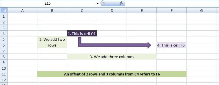
OFFSET returns a reference to a cell or a range of cells using another cell as starting point. A simple example will make this clear: suppose you're in cell C4. An offset of 2 rows and 3 columns brings you to cell F6, there column F is 3 columns further away from column C and row 6 is 2 rows down row 4.


The same can be obtained with ranges. Suppose your current range is A5:L5, an offset of 4 rows would refer to range A9:L9.

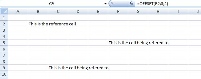
This is basically what the OFFSET function does, returning a reference to a cell or range of cells that is some rows and columns away from another cell or range of cells. To be more specific, have a look at the example below:


Cell B2 is our reference cell, our "starting point". Cell C9 contains the Offset function as can be seen in the formula bar, using cell B2 as initial reference and adding 3 rows and 4 columns. The cell being referenced to is thus cell F5. As cell C9 is as we now know referring to cell F5 through the OFFSET function, the value of F5 is shown in C9. It is as simple as that.

And it works with ranges as well. Cell B7 contains the OFFSET function, Range B2:J2 is our start range and we need to reference the range that is 2 rows below:


Pressing F9 in the formula field will indeed show the offset is refering to the entire range and not just a single cell, although only the first range value is shown in cell B7:


OK, got that. But what is the link with a dynamic chart?

Dynamic Charts

Have a look at our table below. Each row contains monthly sales figures for one trader. It would be nice if I could select a trader, automatically refer to the range containing the trader's sales data, and plot that data on a chart.


I think I start to understand. Using the OFFSET function, you'll refer to the range containg the right data. But the question is, how to use the function and how will the OFFSET function know I need to view Tom's or Megan's or any other trader's data?

That actually is a piece of cake. There're plenty of possibilities to do that. Let me again explain the OFFSET function in detail first. In its most simple form, the one we'll use in this example, the function takes three parameters:

a. The reference cell or range of cells, being the cell or range of cells we'll use as starting point
b. The number of rows, up or down, that we want to refer to.
c. The number of columns, left or right, that we want to refer to.

So basically, the only thing we need to do is telling the formula that the reference range is a certain table row, e.g. the header row, and telling that Tom is one row below, Megan 2, Ben 3 etc.

I know, I know! We can use the MATCH function. MATCH will return the relative position of an element in the range, so using MATCH for Megan on the first table column will return 3. Using this in my OFFSET function will return the range I want.

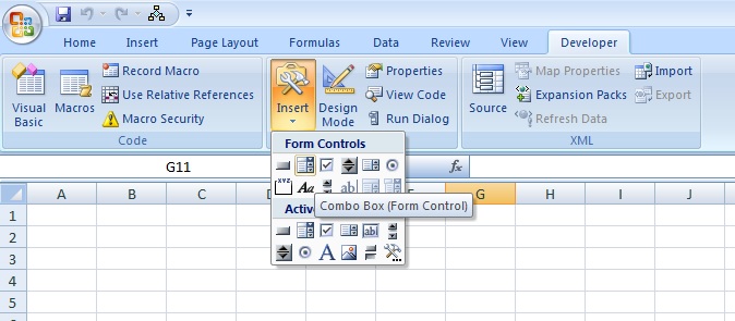
Alright, you're getting good at this. That is one very nice possible option. Myself however I decided to use a Combo Box. Inserting a Combo Box can be done via the Developer's menu:


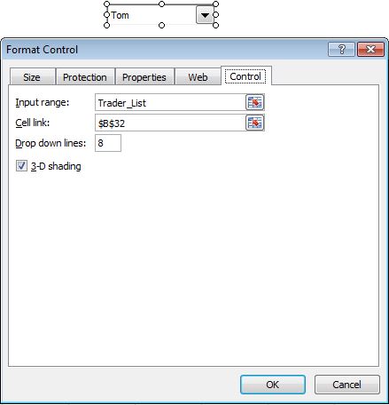
After a right mouse click on the control itself, you're able to modify the Combox Controls:


Two parameters are important in our case:

1. The input range. This is where the Combo Box gets its values from. I've here defined a Named Range called Trader_List that is referring to the first table column
2. A cell link, in this example cell B32. In this cell, Excel will store the relative position of the selected item in the ComboBox. Selecting "Megan" in the Combo Box will return value 2 in cell B32 as Megan is the second trader of the list.

And it is that value you'll use in your OFFSET function!

Exactly!

But how do you tell the chart?

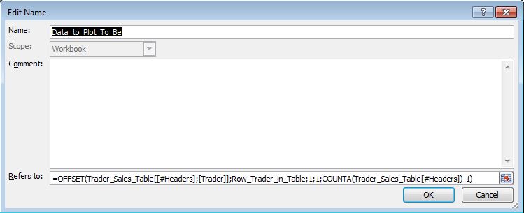
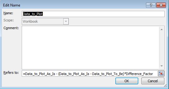
Well that's not too complicated either. I just defined a named range called "Data_to_plot_To_Be" as such:


Oh my goodness! Not complicated you said?

Let's go through it step by step:

1. The first part of the formula is our reference cell: Trader_Sales_Table[[#Headers];[Trader]], which is just the upper left cell of our table. If you need some help in using table cells, table ranges or named ranges, just let me know, my contact details can be found below. Instead of using Trader_Sales_Table[[#Headers];[Trader]], you could just have used B22. If you however later on decide to move the table, referencing to B22 will not work any more whereas your table reference will still be valid.

2. Row_Trader_in_Table is a named range refering to cell B32, if you remember well the "Cell Link" of our Combo Box". This will be our row OFFSET. Again, you could just have used B32 instead.

3. 1 is our column OFFSET. The actual data indeed starts in column C whereas our reference cell is in column B, so we need to shift 1 column to the right.

We now as well introduce 2 optional parameters to our Offset function, that are used if the returned reference has a different heigth and width than the initial reference. Our initial reference is just one cell, we however need the 12 months sales values to be returned. That is why:

4. The fourth parameter is 1, as we just need one row;
5. The fifth parameter is 12.

12? I'm more reading something like COUNTA(Trader_Sales_Table[#Headers])-1

Which turns out to be exactly 12. COUNTA will count the number of non empty cells in the header row of our Trader_Sales_Table table. We need to remove 1 there, as you see, our table as 13 columns and not 12...

Well, it is more complicated than I thought...

These are good practices. The good thing is that it will still work if you decide to add another trader, or analyse the data over 24 instead of 12 months, and this without changing anything to your formulas.

And now it works?

Sure.

I still don't have a chart...

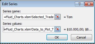
Well, just add one! And for you data series, just refer to the named range we created here above: Data_to_plot_To_Be. You'll need to put the workbook name in front or it will not work.


When you're selecting another trader in the Combo Box, the value of cell B32 (named Row_Trader_in_Table) will change. Therefore, as that cell is used in the OFFSET function of the Data_to_Plot_To_Be named range, the chart will show the corresponding data.


Animated charts

Let's now add some nice animated transitions between the different data sets.

So, I'm just starting to understand the above and you'll start confusing me again...

Just don't listen if you're not interested.

I can't, I'm stuck in this webpage remember? I cannot escape!

I'll do my best to be as clear and concise as possible.

And I'll do my best to be as constructive and invisible as possible.

Animating a chart is not that difficult, but it requires some Visual Basic programming. Luckily, I did the job for you. The algorithm is pretty short and looks as follow:

1. Define in how many transition steps you want to animate your chart and store that in a variable, or let a named range refer to that value in your worksheet (this is actually what I did, the range is named "Smoothness"). For example, suppose one of your old chart value is 0 and the new value is 100. You could bridge the gap in 10 steps, being 10, 20, 30, 40, 50, 60, 70, 80, 90 and 100. Or you could bridge the gap in 100 steps: 1, 2, 3, ... 100. That last one will be much smoother but will be slower. It is a choice to be made;

2. Store the current chart values in a variable, or have a named range refer to them. Again this what I did. I store the previously selected trader in the worksheet and use that value to retrieve the old values in the range Data_to_Plot_As_Is;

3. Store the new chart values in a variable, or have a named range refer to them. This is what we did in the dynamic chart thing, our new data can be referred to via Data_to_Plot_To_Be;

4. The data that will be shown on the chart won't be, unlike in the dynamic chart examples, the Data_to_Plot_To_Be referred values, but will be contained in a new named range called Data_to_Plot. Per "Smoothness step" the Data_to_Plot values will be updated, starting from Data_to_Plot_As_Is and ending at Data_to_Plot_To_Be.


The difference_factor will be updated at each iteration as such:


OK, I see. Your starting point is the As_Is data range. The more the i variable approaches your Smoothness, the more the data to plot will near the To_Be data range.

And what's the DoEvents command doing?


It interrupts the loop and gives back the hand to your operating system, allowing it for instance to process keys that would have been pressed, but allowing it as well to update the chart.

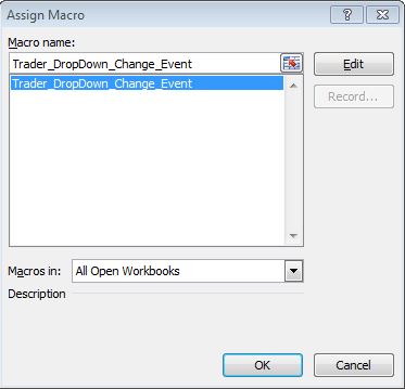
The last thing you need to do is assign the macro that you created to a change in your dropdown. You can do that via a right mouse click on the dropdown itself:


And there you go! The download link containing these examples as well as the VBA code is right here.


Good to know, and to remember...

  • CTRL + F3 will show you the name manager screen so you can immediately see what defined names are used in your document;

  • When using named ranges as your chart data, you always need to put in front your workbook name in order for it to work: Fluid_Charts.xlsm!Data_to_Plot_To_Be;

  • Don't forget the DoEvents function to briefly yield the operating system;


We appreciate your feedback!


About Cintellis

Let us surprise you with how much more you can achieve by using Excel and VBA based products.

Are you looking for an on the level, reliable and trustworthy company that will surprise you with how much more you can achieve by using Excel and VBA based products? Learn more about our philosophy, products, services or contact us for more info.


About Numis

Flexible, cheap and very short implementation time, discover Numis, our Excel based Cash Management and Management Accounting Software and experience a totally new way to analyse and report on your cash positions.

At Numis, we help you to get more out of your financial data than you thought possible. From enhanced reporting functionalities and detailed analysis to providing enterprise budgeting and forecasting solutions, we will help you to achieve your business objectives. When using Numis, you can share your analysis and strategy with your business partners, suppliers or employees as needed.

Numis is a product from Cintellis bvba & FS&P bvba.

CONTACT Us

You can contact us by phone, mail or by filling out the form below.

Corporate address:
Alsembergsesteenweg 588
1653 Dworp
Belgium

Phone Numbers:
+32 (0)471 65 19 66

E-Mail: info@cintellis.com